Advanced operations - Calibration Table Tab

 

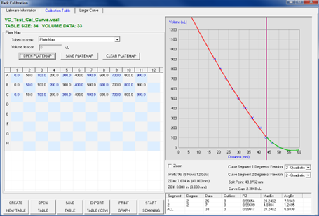
Use the Calibration Table tab to:

• Create plate maps of known volumes to measure (plate maps have a .PMF file extension).
• Scan known volume data for a calibration plot.
• Adjust the measured data with curve fitting tools.
• Save the calibration table (.VCAL file).

Note: Append additional data points to the calibration plot by clearing the plate map and entering new data points to scan to the table.

Calibration table functions

• CREATE NEW TABLE: Creates a new calibration file.
• OPEN TABLE: Opens a previously created calibration file.
• SAVE TABLE: Saves a calibration table. Calibration tables are saved with a .vcal file extension.
• EXPORT TABLE (.CSV): exports the calibration table data in a .CSV file.
• PRINT GRAPH: prints the calibration table graph.
• START SCANNING: Click this button to begin the plate scanning process and for appending
  data points.
• ZOOM: Click and drag the right mouse button over calibration curve data points.
• UNZOOM: Reverses zoom feature.

The Larger Curve tab provides an enhanced view of the calibration data table.

Creating a plate map

For this example, the calibration table is based on a well plate using a limited number of known
sample volumes (0, 50, 100, 200, 300, 400, …..). The software uses a plate map of the sample
volume values to associate the sample volume with the well location.

Typically, a larger number of samples are needed (see recommended calibration plot sample data below). The software will generate a calibration plot of sensor-to-sample liquid level in the well plate. The software curve fitting features are used to fit calibration curve segments to the data. With the curve fitted to the data, the calibration data is saved as a calibration table.

1. Under the Tubes to Scan drop down menu, make a convenient selection.
2. Under the Volume to Scan window, enter a volume to populate the Tube to Scan selection or
   manually enter values in each cell of the plate map.
3. OPEN PLATE MAP – you can create a plate map as a .csv file and import it into the
   VolumeCheck plate map, if you prefer.

Note: the VolumeCheck USB Flash Drive includes example plate map files.

Recommended Calibration Plot sample data

• For best volume measurement results, sample volumes used to create the calibration table
  should be in small increments (10µL to 20µL) for the lower volumes of the well and larger
  increments (25µL to 50µL) for the higher volumes of the well.
• To save time and reduce the number of samples, most wells and tubes can be measured
  using 10 to 20µL increments for the first 0µL - 100µL of volume (this usually fills the conical
  portion of the tube), then as the well shape becomes more linear, the sample increments can be increased to 50µL - 100µL increments. As the well shape becomes more linear; the
  resulting calibration plot also becomes more linear. Prior to creating a calibration table with
  10µL to 20µL sample increments, it is recommended to first make a test calibration table
  using 25µL to 50µL or larger increments to establish a general understanding of labware
  characteristics in the low and high volume areas.

Set up the plate map

The calibration table page displays a plate map showing e.g. the well layout of a 96-tube SBS plate, if this is what you had set up. The plate map is used to associate the sample volume amount with the well location.

For this example, enter the following example data into the plate map grid:

Next, dispense the sample volume into the well plate to match the above values.

Note: the seven sample volumes in 50µL increments (0 to 300µL) used in this example will create calibration table that may be limited in accuracy.

For new labware or samples, to get a general idea of labware characteristics in the low and high volume areas, SPT Labtech recommends that several test calibration tables are made using 25µL to 50µL or larger increments.

This is the output from the initial calibration plot (left) and plot curve fitted to create a Calibration
Table (right).

Start scanning for calibration table data

1. Place the well plate onto VolumeCheck input tray (A01 to the back of tray).
2. Click on the Start Scanning button.
3. VolumeCheck will scan the well plate and take sensor-to-sample distance measurements.
4. The measurement data is shown plotted in the graph window.

Use The Software Curve Matching Tools Features To Fit The Data To The Curve

• The curve can be divided into two segments (use the mouse to move the red plot divider line
  to break the plot into two segments. This red line is located on the right side of the graph
  window).
• Use the Degree of Freedom selector to choose the best type of fit for the plot segment.

Typical Settings: 

• If using a single segment curve: use Linear.
• If using two segments: use linear curve fit setting for the higher volume segment and quadratic curve fit setting for the lower volume segment.
• For 384-wellplates, a single segment curve with cubic fit is common.

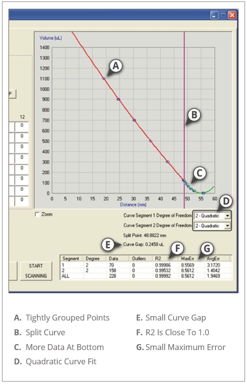
The Data Point Information Screen – Curve fitting & Calibration table

The Data Point Information Screen allows you to select data points to be included or excluded
from the calibration table.

Due to labware and sample characteristics, there may be some data points that fall outside of the
curve of the calibration table. These outlying data points can be included or excluded from the final calibration curve. Select outlying data points by double-clicking on the point. The Data Point
Information screen displays with the selected data points. Check or uncheck the numbered box to the left in order to include or exclude data points from the calibration curve.

Calibration plot with outlier point (left) & plot with outlier point deselected (right).

Note: Data Point Information is not deleted when excluded. You can always re-include data points via the Data Point Information screen.

After the calibration table has been fine-tuned, save the calibration table, by clicking the Save
Table button. The software will prompt you for a file name. The calibration table file extension is
.vcal.

Note: It may be helpful to name calibration curves by the labware type, well size, and sample type.

Selecting and deselecting data points (deselecting outliers & out of range data points)

Data points can be selected and deselected by:

• Clicking on individual data points, or
• Dragging the cursor over a plot area to select a group of data points.

Deselecting outlier data points can improve the fit of the data to the curve.

Fitting a curve to the data

• Maximum error (in µL volume) is shown in the box on the bottom of the screen for each
  curve segment.
• Changing the degree of freedom and deselecting outlier points can be used to reduce the
  amount of maximum error.
• Results are dependent on type of labware and sample, but achievable values (for typical 1mL size tube/well) are:
  • Split Point: The point on the curve where the degree of freedom changes.
  • Curve Gap: Set to as low a value as possible.
  • AvgErr: adjust to less than 10µL.
  • MaxErr: adjust to less than 15µL.
  • R2: Goal is as close to one (1.0) as possible.

Note: Good curves typically have 8-12 data points at each volume dispense. This is dependent on the overall volume of the well.

Outlier data points can be caused by a variety of reasons including:

• Improper meniscus detection due to droplets on the side of the well, or bubbles in sample,
  etc.
• The plate map entered value does not match the dispensed sample volume (example: plate
  map value for A01 is 100µL, but 300µL was dispensed into A01 which generates an
  unexpected outlier data point).

Characteristics of a good calibration curve

 

Tips:

A. Tightly grouped points: SPT Labtech recommends that you measure multiple wells containing
the same volume. Ideally, these points will be distributed across a rack (for example, A01, A02, …, A12) to better represent all positions on the rack. A distribution of 0.5mm or less is considered
very good; a 1mm limit is recommended.

B. Split curve: For most labware, geometry at the tip (or bottom of the well) will differ from
geometry along the length (or upper portion) of the tube. The calibration curve is split to better fit
both geometries.

C. More data at tube/well bottom: For 96 well individual tubes (e.g. Matrix or Micronic), SPT
Labtech recommends you collect data at 10µL increments at the bottom (0-100µL for example).
After the sample meniscus is above the tip-to-cylinder transition, you may increase the volume
increments.

D. Quadratic curve fit: In general, a quadratic curve fit works best for both segments of the
curve. This is especially true at the tip (segment 2, shown in green). For some labware, a cubic
curve fit may more closely follow the data points.

E. Small curve gap: A curve gap exists at the junction between two curve segments. It is possible to see this gap if you zoom in at the junction (see below). Slide the vertical purple divider until your curve gap is less than 1µL (you may have to zoom in at the junction).

F. R2 close to 1.0: R2, the correlation coefficient, should usually be greater than 0.99, no less than 0.95.

G. Small maximum error: The maximum error indicates the accuracy of the calibration curve. It
is determined by the outlier that is most distant from the fitted curve. While it is possible to exclude outliers, try to gather data that clusters tightly. For individual tubes, like Matrix and Micronic tubes, maximum error should be below 15µL. With careful fluid dispensing and uniform sample dispenses, it is possible to limit error to less than 10µL. Labware with larger diameters, like 2.0mL vials, will inherently have larger error, so the error limit may be increased to 20µL.

At this point your calibration table should be saved.

• Click the Save Table button to name and save the table.

Exit Plate Data Creator Tool

• Click on X in the upper right of the screen to exit and return to the main screen.

Loading the Calibration Table and testing VolumeCheck

From Main Screen of the VolumeCheck program.

1. Click on the Load Table button and select the example calibration table that was just created.
2. Load the plate into the VolumeCheck input tray.
3. Click on the Start button.
4. VolumeCheck scans the plate and displays volume data on-screen.
5. The volume data for the plate should correspond to the well volume.
6. If adjustment to the calibration table is needed (e.g. changes in curve fitting) go to the Plate
   Data Creator tool to make adjustments and save the updated table under a new name for
   testing.

Saving Project Files

The project feature allows saving software settings (calibration file, error handling, display settings, etc.) for future use. Before saving a project, load the appropriate calibration table so it is
associated with the project.

Note: this only saves the association of the calibration table to the Project file; it does not save or make a copy of the calibration table file.

• To save and name a Project, click on File Menu, Save Project.
• The project can now be used in the future.
• Click on the File Menu, Load Project to select a saved project.
• The project file workflow bundles the calibration table, software display settings, and error
  handling to simplify using multiple labware types with different software settings.